Temporal Point Processes 2: Neural TPP Models
How can we define flexible TPP models using neural networks?
In this post, we will learn about neural temporal point processes (TPPs) — flexible generative models for variable-length event sequences in continuous time. More specifically, we will
- Learn how to parametrize TPPs using neural networks;
- Derive the likelihood function for TPPs (that we will use as the training objective for our model);
- Implement a neural TPP model in PyTorch.
If you haven’t read the previous post in the series, I recommend checking it out to get familiar with the main concepts and notation. Alternatively, click on the arrow below to see a short recap of the basics.
Recap
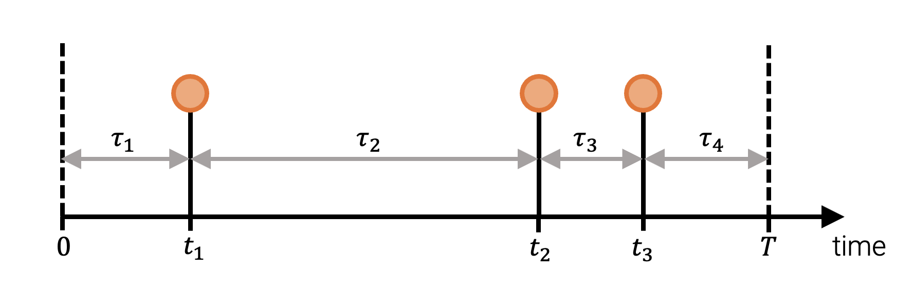
A temporal point process (TPP) is a probability distribution over variable-length event sequnces in a time interval $[0, T]$. We can represent a realization of a TPP as a sequence of strcitly increasing arrival times $\boldsymbol{t} = (t_1, ..., t_N)$, where $N$, the number of events, is itself a random variable. We can specify a TPP by defining $P_i^*(t_i)$, the conditional distribution of the next arrival time $t_i$ given past events $\{t_1, \dots, t_{i-1}\}$, for $i = 1, 2, 3, \dots$. The distribution $P_i^*(t_i)$ can be specified with either a probability density function (PDF) $f_i^*$, a survival function (SF) $S_i^*$, or a hazard function (HF) $h_i^*$.Representing the data
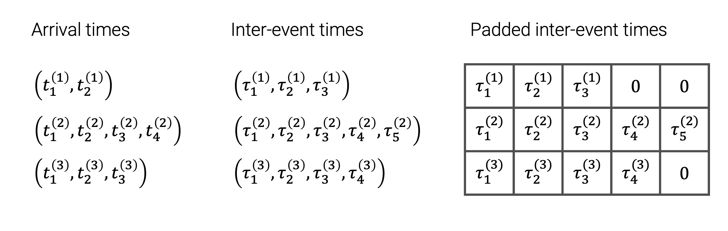
We will define our neural TPP as an autoregressive model. To do this, at each step $i = 1, 2, 3, …$ we need to specify the distribution \(P_i^*(t_i) := P_i(t_i \vert \mathcal{H}_{t_i})\) of the next arrival time \(t_i\) given the history of past events \(\mathcal{H}_{t_i} = \{t_1, \dots, t_{i-1}\}\). An equivalent but more convenient approach is to instead work with the inter-event times $(\tau_1, \dots, \tau_{N+1})$,
First, let’s load some data and covnert it into a format that can be processed by our model. You can find the dataset and a Jupyter notebook with all the code used in this blog post here.
Constructing a neural TPP model
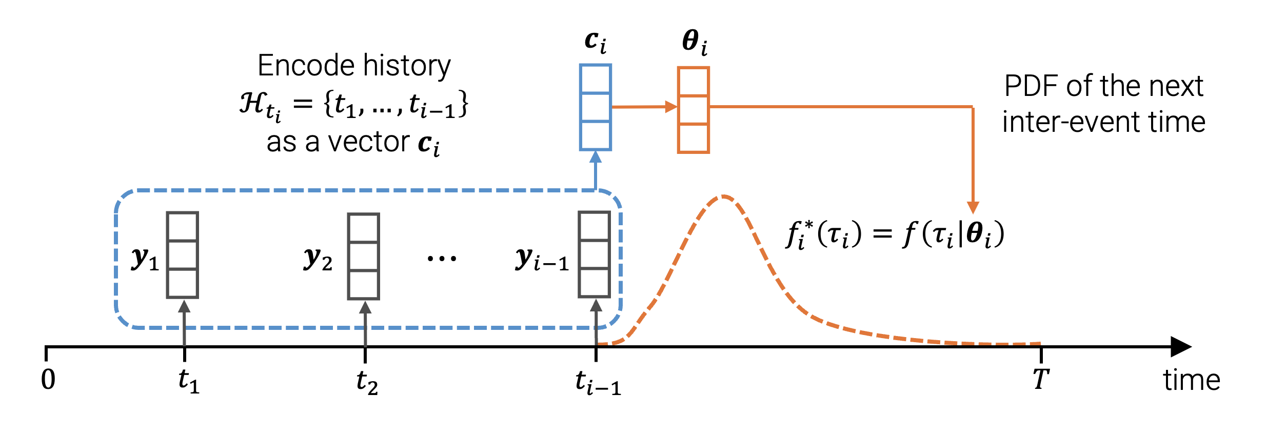
How can we parametrize the conditional distribution \(P_i^*(\tau_i)\) with a neural network? A simple and elegant answer to this question was proposed in the seminal work by Du, Dai, Trivedi, Gomez-Rodriguez and Song
- Encode the event history \(\mathcal{H}_{t_i} = \{t_1, \dots, t_{i-1}\}\) into a fixed-dimensional context vector \(\boldsymbol{c}_i \in \mathbb{R}^C\) using a neural network.
- Pick a parametric probability density function \(f(\cdot \vert \boldsymbol{\theta})\) that defines the distribution of a positive
We always assume that the arrival times are sorted, that is, $t_i < t_{i+1}$ for all $i$. Therefore, the inter-event times $\tau_i$ are strictly positive. random variable (e.g., PDF of the exponential distribution or Weibull distribution). - Use the context vector \(\boldsymbol{c}_i\) to obtain the parameters \(\boldsymbol{\theta}_i\). Plug in \(\boldsymbol{\theta}_i\) into \(f(\cdot \vert \boldsymbol{\theta})\) to obtain the PDF \(f(\tau_i \vert \boldsymbol{\theta}_i)\) of the conditional distribution \(P_i^*(\tau_i)\).
We will now look at each of these steps in more detail.
Encoding the history into a vector
The original approach by Du et al.
- Each event $t_j$ is represented by a feature vector $\boldsymbol{y}_j$. In our model, we will simply define $\boldsymbol{y}_j = (\tau_j, \log \tau_j)^T$.
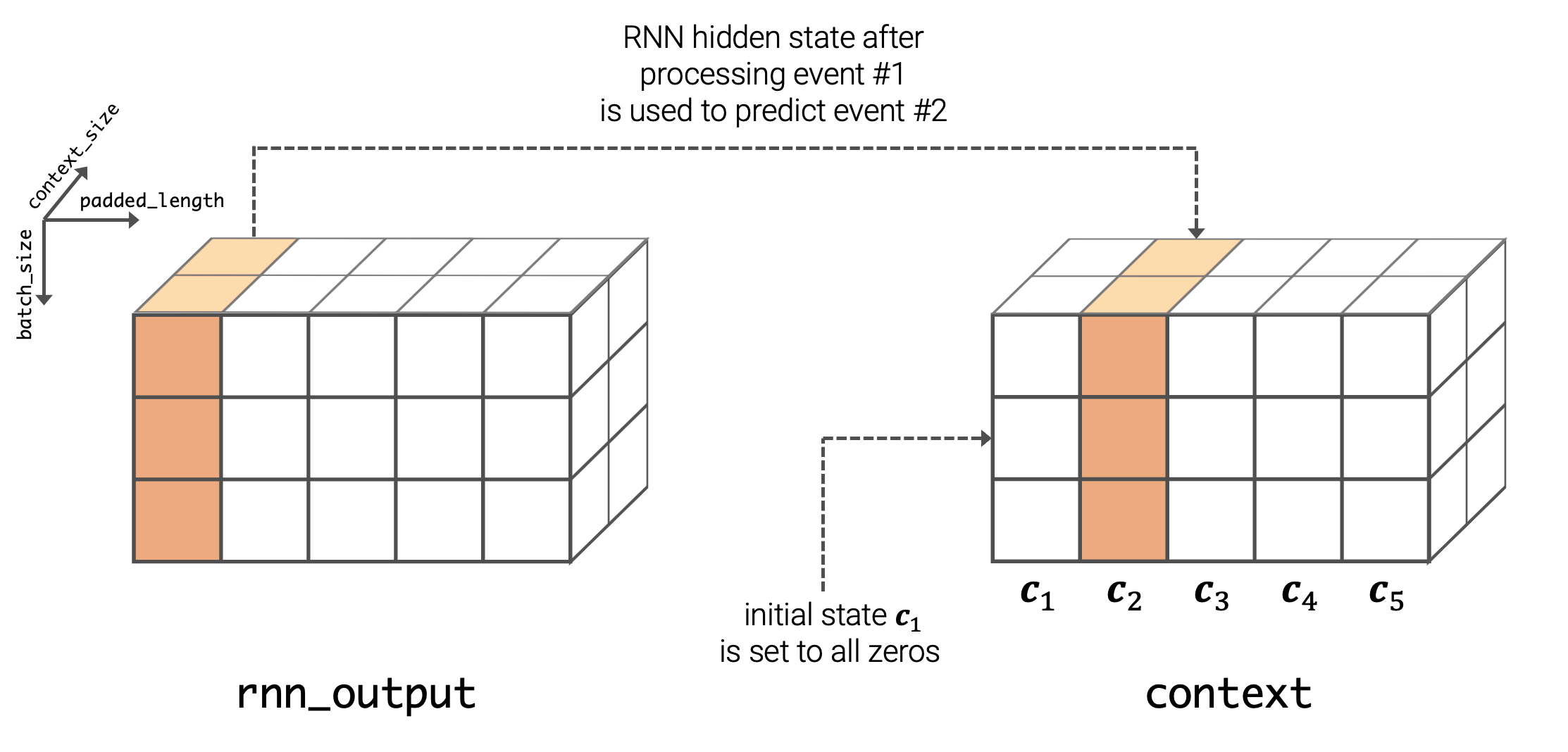
Using the logarithm here allows the model to distinguish between very small inter-event times. More sophisticated approaches, like positional encoding with trigonometric functions, are also possible. - We initialize $\boldsymbol{c}_1$ (for example, to a vector of all zeros). The vector $\boldsymbol{c}_1$ will work both as the initial state of the RNN, as well as to obtain the parameters of $P_1^*(\tau_1)$.
- After each event $t_i$, we compute the next the context vector $\boldsymbol{c}_{i+1}$ (i.e., the next hidden state of the RNN) based on the previous state $\boldsymbol{c}_i$ and features $\boldsymbol{y}_i$ $$ \boldsymbol{c}_{i+1} = \operatorname{Update}(\boldsymbol{c}_i, \boldsymbol{y}_{i}). $$ The specific RNN architecture is not very important here — vanilla RNN, GRU or LSTM update functions can all be used here. By processing the entire sequence $(t_1, \dots, t_N)$, we compute all the context vectors $(\boldsymbol{c}_1, \dots, \boldsymbol{c}_{N+1})$.
Choosing a parametric distribution
When picking a parametric distribution for inter-event times, we have to make sure that its probability density function (PDF) $f(\cdot \vert \boldsymbol{\theta})$ and survival function $S(\cdot \vert \boldsymbol{\theta})$ can be computed analytically — we will need this later when computing the log-likelihood. For some applications, it’s also nice to able to sample from the distribution analytically. I decided to use Weibull distribution here as it satisfies all these properties.
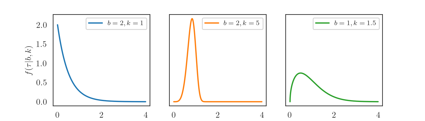
The Weibull distribution has two strictly positive parameters $\boldsymbol{\theta} = (b, k)$. The probability density function is computed as \[ f(\tau \vert b, k) = b k \tau^{k-1} \exp(-b \tau^{k}) \] and the survival function is \[ S(\tau \vert b, k) = \exp(-b \tau^{k}). \]
We implement the Weibull distribution using an API that is similar to torch.distributions.
Conditional distribution
To obtain the conditional PDF $f^*_i(\tau_i) := f(\tau_i | k_i, b_i)$ of the next inter-event time given the history, we compute the parameters $k_i$, $b_i$ using the most recent context embedding $\boldsymbol{c}_i$ \[ \begin{aligned} k_i = \sigma(\boldsymbol{v}^T_k \boldsymbol{c}_i + d_k) & \qquad & b_i = \sigma(\boldsymbol{v}^T_b \boldsymbol{c}_i + d_b). \end{aligned} \] Here, $\boldsymbol{v}_k \in \mathbb{R}^C, \boldsymbol{v}_b \in \mathbb{R}^C, d_k \in \mathbb{R}, d_b \in \mathbb{R}$ are learnable weights, and $\sigma: \mathbb{R} \to (0, \infty)$ is a nonlinear function that ensures that the parameters are strictly positive (e.g., softplus).
The weights $\{\boldsymbol{v}_k, \boldsymbol{v}_b, d_k, d_b\}$ together with the weights of the RNN are the learnable parameters of our neural TPP model. The next question we have to answer is how to estimate these from data.
Likelihood function
Log-likelihood (LL) is the default training objective for generative probabilistic models, and TPPs are no exception. To derive the likelihood function for a TPP we will start with a simple example.
Suppose we have observed a single event with arrival time \(t_1\) in the time interval \([0, T]\). We can describe this outcome as “the first event happened in $[t_1, t_1 + dt)$ and the second event happened after $T$”.
The equality here follows simply from the definition of the PDF \(f_1^*\) and the survival function \(S_2^*\) (as discussed in the previous post).
The $(dt)^N$ term is just a multiplicative constant with respect to the model parameters, so we ignore it during optimization. By taking the logarithm, we get the log-likelihood
\[\begin{align} \log p(\boldsymbol{t}) &= \left(\sum_{i=1}^{N} \log f_i^*(t_i)\right) + \log S_{N+1}^*(T). \end{align}\]Lastly, by slightly abusing the notation, we switch back to the inter-event times and obtain
\[\begin{align} \log p(\boldsymbol{t}) &= \left(\sum_{i=1}^{N} \log f_i^*(\tau_i)\right) + \log S_{N+1}^*(\tau_{N+1}). \end{align}\]We will use this formulation of the log-likelihood to train our neural TPP model.
It’s worth noting that Equation (4) is not the only way to express the log-likelihood of a TPP. In the previous post, we talked about different functions characterizing a TPP, such as conditional hazard functions \(\{h_1^*, h_2^*, h_3^*...\}\) and the conditional intensity function \(\lambda^*(t)\). Many papers and textbooks work with these functions instead. Click on the arrow below for more details.
Other ways to compute the log-likelihood of a TPP
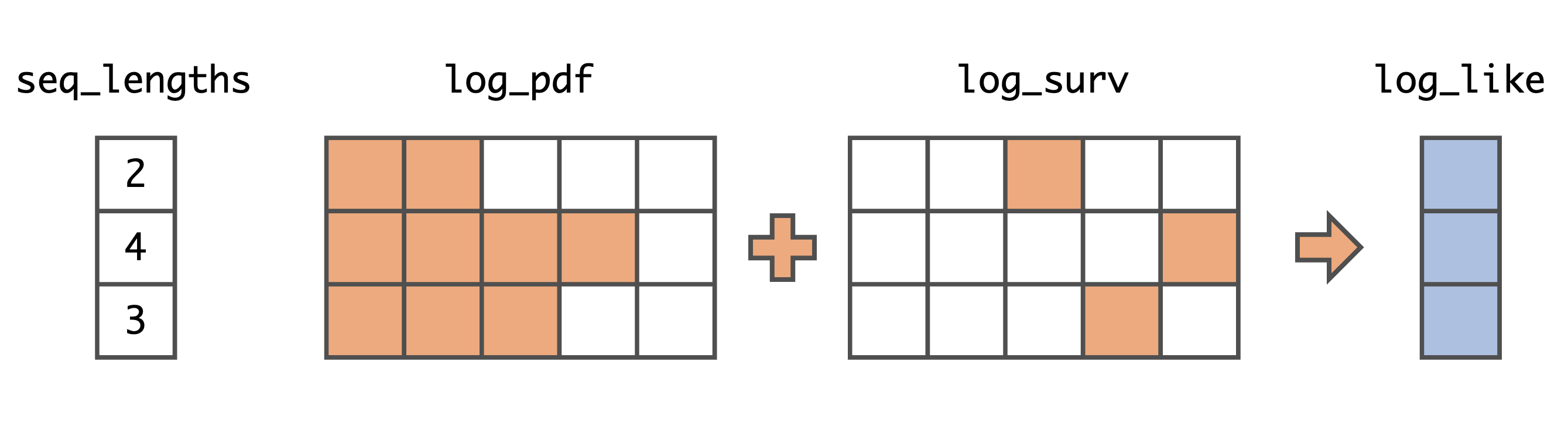
We combine Equation (3) with the definition of the conditional hazard function $h_i^*(t) = f_i^*(t)/S_i^*(t)$ and obtain $$ \begin{aligned} \log p(\boldsymbol{t}) =& \left(\sum_{i=1}^{N} \log f_i^*(t_i)\right) + \log S_{N+1}^*(T)\\ =& \left(\sum_{i=1}^{N} \log h_i^*(t_i) + \log S_i^*(t_i)\right) + \log S_{N+1}^*(T)\\ =& \sum_{i=1}^{N} \log h_i^*(t_i) + \sum_{i=1}^{N+1} \log S_i^*(t_i), \end{aligned} $$ where we defined $t_{N+1}=T$. Last time, we derived the equalityThe trickiest part when implementing TPP models is vectorizing the operations on variable-length sequences (i.e., avoiding for-loops). This is usually done with masking and operations like torch.gather. For example, here is a vectorized implementation of the negative log-likelihood (NLL) for our neural TPP model.
Putting everything together
Now we have all the pieces necessary to define and train our model. Here is a link to the Jupyter notebook with all the code we’ve seen so far, but where the different model components are nicely wrapped into a single nn.Module.
As mentioned before, we train the model by minimizing the NLL of the training sequences. More specifically, we average the loss over all sequences and normalize it by $T$, the length of the observed time interval.
There are different ways to evaluate TPP models. Here, I chose to visualize some properties of the event sequences generated by the model and compare them to those of the training data. The code for sampling is not particularly interesting. It follows the same logic as before — at each step $i$, we sample the next inter-event time $\tau_i \sim f_i^*(\tau_i)$, feed it into the RNN to obtain the next context embedding $\boldsymbol{c}_{i+1}$, and repeat the procedure. See the Jupyter notebook for details.
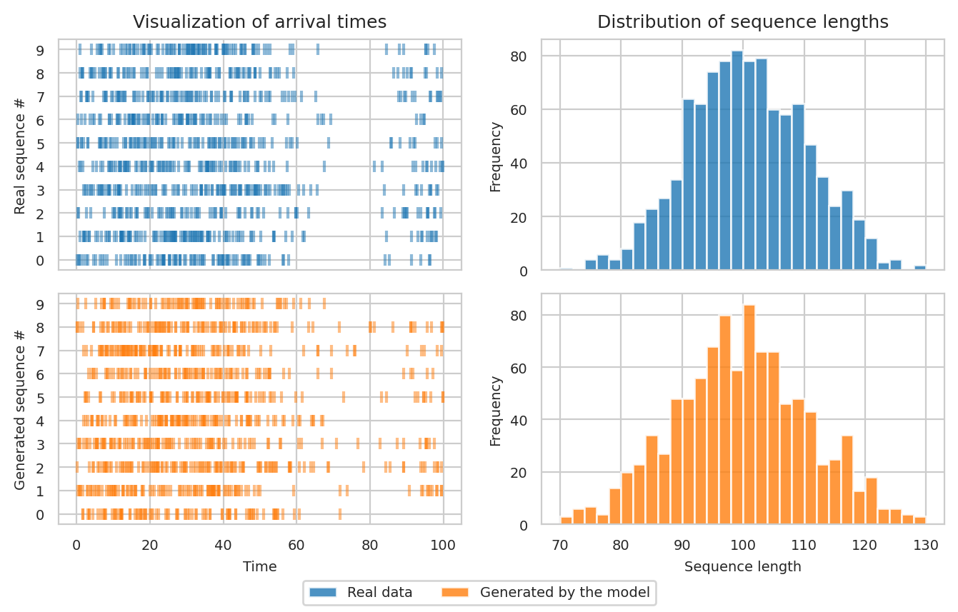
Left: Visualization of the arrival times in 10 real (top) and 10 simulated (bottom) sequences.
Right: Distribution of sequence lengths for real (top) and simulated (bottom) event sequences.
We see that training sequences have a trend: there are a lot more events in the $[0, 50]$ interval than in $[50, 100]$ (top left figure). Our neural TPP model has learned to produce sequences with a similar property (bottom left). The figure also shows that the distribution of the sequence lengths in real (top right) and simulated (bottom right) sequences are quite similar. We conclude that the model has approximated the true data-generating TPP reasonably well. Of course, there is room for improvement. After all, we defined a really simple architecture, and it’s possible to get even better results by using a more flexible model.
Concluding remarks
In this post, we have learned about the general design principles of neural TPPs and implemented a simple model of this class. Unlike traditional TPP models that we discussed in the previous post (Poisson processes, Hawkes processes), neural TPPs can simultaneously capture different patterns in the data (e.g., global trends, burstiness, repeating subsequences).
Neural TPPs are a hot research topic, and a number of improvements have been proposed in the last couple of years. For example, one can use a transformer as the history encoder
So far we have been talking exclusively about the so-called unmarked TPPs, where each event is represented only by its arrival time $t_i$. Next time, I will talk about the important case of marked TPPs, where events come with additional information, such as class labels or spatial locations.
Acknowledgments
I would like to thank Daniel Zügner for his feedback on this post.