Temporal Point Processes 1: The Conditional Intensity Function
How can we define generative models for variable-length event sequences in continuous time?
TL;DR
- Temporal point processes (TPPs) are probability distributions over variable-length event sequences in continuous time.
- We can view a TPP as an autoregressive model or as a counting process.
- The conditional intensity function $\lambda^*(t)$ connects these two viewpoints and allows us to specify TPPs with different behaviors, such as a global trend or burstiness.
- The conditional intensity $\lambda^*(t)$ is one of many ways to define a TPP — as an alternative, we could, for example, specify the conditional PDFs of the arrival times \(\{f_1^*, f_2^*, f_3^*, ...\}\).
What is a point process?
Probabilistic generative models are the bread and butter of modern machine learning. They allow us to make predictions, find anomalies and learn useful representations of the data. Most of the time, applying the generative model involves learning the probability distribution \(P(\boldsymbol{x})\) over our data points \(\boldsymbol{x}\).
We know what to do if \(\boldsymbol{x}\) is a vector in \(\mathbb{R}^D\) — simply use a multivariate Gaussian or, if we need something more flexible, our favorite normalizing flow model. But what if a single realization of our probabilistic model corresponds to a set of vectors \(\{\boldsymbol{x}_1, ..., \boldsymbol{x}_N\}\)? Even worse, what if both \(N\), the number of the vectors, as well as their locations \(\boldsymbol{x}_i\) are random? This is not some hypothetical scenario — processes generating such data are abundant in the real world:
- Transactions generated each day in a financial system
- Locations of disease outbreaks in a city, recorded each week
- Times and locations of earthquakes in some geographic region within a year
Point processes provide a framework for modeling and analyzing such data. Each realization of a point process is a set \(\{\boldsymbol{x}_1, \dots, \boldsymbol{x}_N\}\) consisting of a random number \(N\) of points \(\boldsymbol{x}_i\) that live in some space \(\mathcal{X}\), hence the name “point process”. Depending on the choice of the space \(\mathcal{X}\), we distinguish among different types of point processes. For example, \(\mathcal{X} \subseteq \mathbb{R}^D\) corresponds to a so-called spatial point process, where every point \(\boldsymbol{x}_i\) can be viewed as a random location in space (e.g., a location of a disease outbreak).
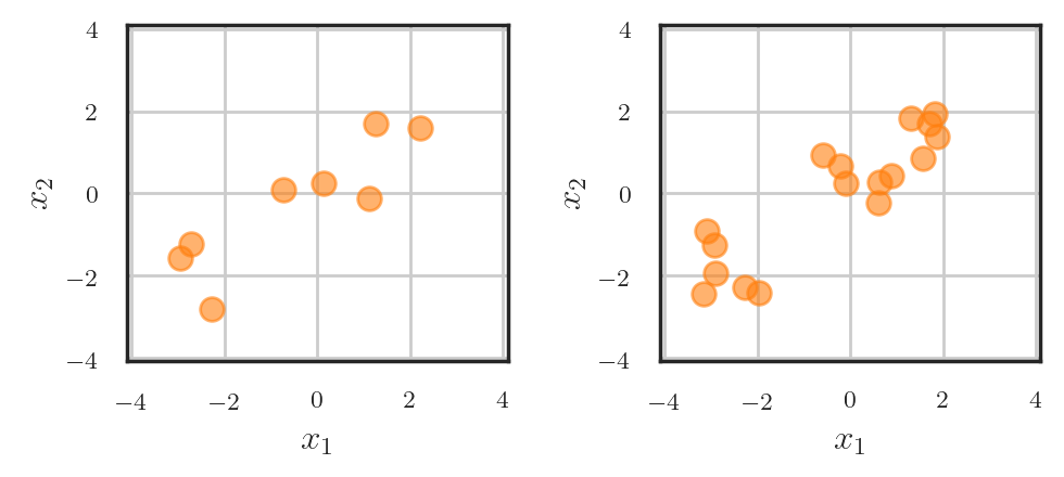
Another important case, to which I will dedicate the rest of this post (and, hopefully, several future ones), are temporal point processes (TPPs), defined on the real half-line \(\mathcal{X} \subseteq [0, \infty)\). We can interpret the points in a TPP as events happening in continuous time, and therefore usually denote them as \(t_i\) (instead of \(\boldsymbol{x}_i\)).
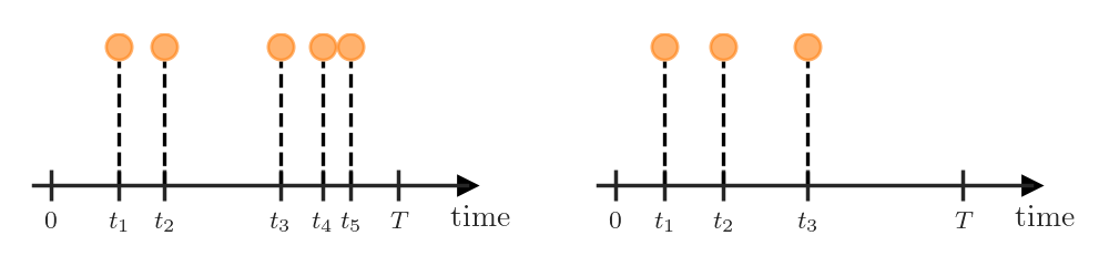
At first it might seem like TPPs are just a (boring) special case of spatial point processes, but this is not true. Because of the ordered structure of the set \([0, \infty)\), we can treat TPP realizations (i.e., sets \(\{t_1, \dots, t_N\}\)) as ordered sequences \(\boldsymbol{t} = (t_1, \dots, t_N)\), where \(t_1 < t_2 < \dots < t_N\). Additionally, we typically assume that the arrival time of the event \(t_i\) is only influenced by the events that happened in the past. As we will see in the next section, this makes specifying TPP distributions rather easy. In contrast, spatial point processes don’t permit such ordering on the events, and because of this often have intractable densities.
The theory of temporal point processes was mostly developed near the middle of the 20th century, taking roots in measure theory and stochastic processes. For this reason, the notation and jargon used in TPP literature may sound strange and unfamiliar to people with a machine learning background (at least it did to me back when I started learning about TPPs). In reality, though, most TPP-related concepts can be easily translated into the familiar language of probabilistic machine learning.
In this post we will investigate different ways to represent a TPP. As we will see, a TPP can be treated as an autoregressive model or as a counting process. We will learn about the conditional intensity function \(\lambda^*(t)\) — a central concept in the theory of point processes — that unites these two perspectives and allows us to compactly describe various TPP distributions.
TPP as an autoregressive model
How do we define a probabilistic model that generates variable-length event sequences \(\boldsymbol{t} = (t_1, \dots, t_N)\)
At each step we are dealing with the conditional distribution of the event \(t_i\) given the history of the past events \(\mathcal{H}_{t_i} = \{t_j: t_j < t_i\}\). We usually denote this distribution as \(P_i(t_i | \mathcal{H}_{t_i})\). In the literature, you will also often meet the shorthand notation \(P_i^*(t_i)\), where the star reminds us of the dependency on past events. The important question is how to represent the probability distribution \(P_i^*(t_i)\).
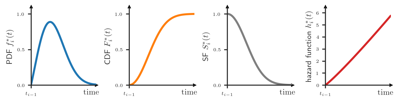
In machine learning, we usually characterize a continuous probability distribution \(P_i^*\) by specifying its probability density functions (PDF) \(f_i^*\). Loosely speaking, the value \(f_i^*(t) dt\) represents the probability that the event \(t_i\) will happen in the interval \([t, t + dt)\), where \(dt\) is some infinitesimal positive number.
However, there exist other ways to describe a distribution that might be more useful in certain contexts. For example, the cumulative distribution function (CDF) \(F_i^*(t) = \int_0^{t} f_i^*(u) du\) tells us the probability that the event \(t_i\) will happen before time \(t\). Closely related is the survival function (SF), defined as \(S_i^*(t) = 1 - F_i^*(t)\), which tells us the probability that the event \(t_i\) will happen after time \(t\).
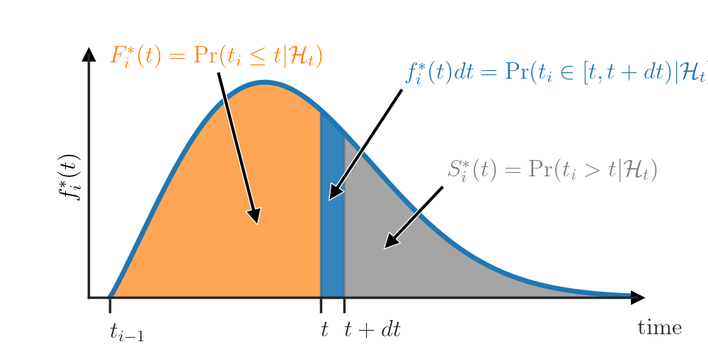
Finally, a lesser known option is the hazard function \(h_i^*\) that can be computed as \(h^*_i(t) = f_i^*(t) / S_i^*(t)\). The value \(h_i^*(t)dt\) answers the question “What is the probability that the event \(t_i\) will happen in the interval \([t, t + dt)\) given that it didn’t happen before \(t\)?”. Let’s look at this definition more closely to examine the connection between the PDF \(f_i^*\) and the hazard function \(h_i^*\).
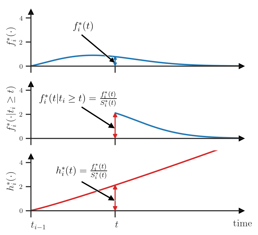
Consider the following scenario. The most recent event \(t_{i-1}\) has just happened and our clock is at time \(t_{i-1}\). The value \(f_i^*(t)dt\) tells us the probability that the next event \(t_i\) will happen in \([t, t+ dt)\) (see next figure — top). Then, some time has elapsed, our clock is now at time \(t\) and the event \(t_{i}\) hasn’t yet happened. At this point in time, \(f_i^*(t)dt\) is not equal to \(\Pr(t_i \in [t, t + dt) | \mathcal{H}_t)\) anymore — we need to condition on the fact that \(t_i\) didn’t happen before \(t\). For this, we renormalize the PDF such that it integrates to \(1\) over the interval \([t, \infty)\) (see next figure — center).
\[f_i^*(t | t_i \ge t) = \frac{f_i^*(t)}{\int_t^\infty f_i^*(u) du} =\frac{f_i^*(t)}{S_i^*(t)} =: h_i^*(t)\]This value of the renormalized PDF exactly corresponds to the hazard function \(h_i^*\) at time \(t\) (see next figure — bottom).
We can also go in the other direction and compute the PDF \(f_i^*\) using \(h_i^*\). First, we need to compute the survival function
\[\begin{aligned} h_i^*(t) &= \frac{f_i^*(t)}{S_i^*(t)} = \frac{- \frac{d}{dt} S_i^*(t)}{S_i^*(t)} = -\frac{d}{dt} \log S_i^*(t)\\ & \Leftrightarrow S_i^*(t) = \exp \left( -\int_{t_{i-1}}^t h_i^*(u) du \right) \end{aligned}\]This, in turn, allows us to obtain the PDF as
\[\begin{aligned} f_i^*(t) &= -\frac{d}{dt}S_i^*(t)\\ & = -\frac{d}{dt}\exp \left( -\int_{t_{i-1}}^t h_i^*(u) du \right)\\ &= h_i^*(t) \exp \left( -\int_{t_{i-1}}^t h_i^*(u) du \right) \end{aligned}\]The name “hazard function” comes from the field of survival analysis, where the goal is to predict hazardous events such as death of a patient or failure of some system. In such a setting, the hazard function \(h_i^*\) is often considered to be more interpretable
Let’s get back to our problem of characterizing the conditional distributions of a TPP. We could specify any of the functions \(f_i^*\), \(F_i^*\), \(S_i^*\) or \(h_i^*\) (subject to the respective constraints
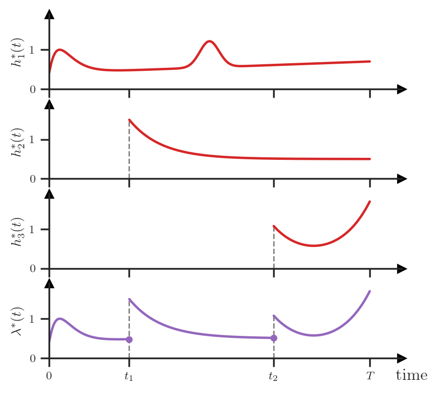
In summary, to define the full distribution of some TPP, we could, for instance, specify the conditional PDFs \(\{f_1^*, f_2^*, f_3^*, \dots\}\) or, equivalently, the conditional hazard functions \(\{h_1^*, h_2^*, h_3^*, \dots\}\). However, dealing with all the different conditional distributions and their indices can be unwieldy. Instead, we could consider yet another way of characterizing the TPP — using the conditional intensity function. The conditional intensity, denoted as \(\lambda^*(t)\), is defined by stitching together the conditional hazard functions:
\[\lambda^*(t) = \begin{cases} h_1^*(t) & \text{ if } 0 \le t \le t_1 \\ h_2^*(t) & \text{ if } t_1 < t \le t_2 \\ & \vdots\\ h_{N+1}^*(t) & \text{ if } t_N < t \le T \\ \end{cases}\]which can graphically be represented as follows:
Let’s take a step back and remember what the \(*\) notation means here. When we write \(\lambda^*(t)\), we actually mean \(\lambda(t | \mathcal{H}_t)\). That is, the conditional intensity function takes as input two arguments: (1) the current time \(t\) and (2) the set of the preceding events \(\mathcal{H}_t\) that can be of arbitrary size.
We can turn the previous statement around: To define a TPP distribution, we simply need to define some non-negative function
Defining TPPs using the conditional intensity function
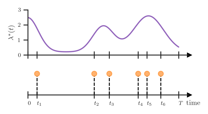
The main advantage of the conditional intensity is that it allows to compactly represent various TPPs with different behaviors. For example, we could define a TPP where the intensity is independent of the history and only depends on the time \(t\).
\[\lambda^*(t) = g(t)\]This corresponds to the famous Poisson process. High values of \(g(t)\) correspond to a higher rate of event occurrence, so the Poisson process allows us to capture global trends. For instance, we could use it to model passenger traffic in a subway network within a day. More events (i.e., ticket purchases) happen in the morning and in the evening compared to the middle of the day, which is reflected by the variations in the intensity \(g(t)\).
The Poisson process has a number of other interesting properties and probably deserves a blog post of its own.
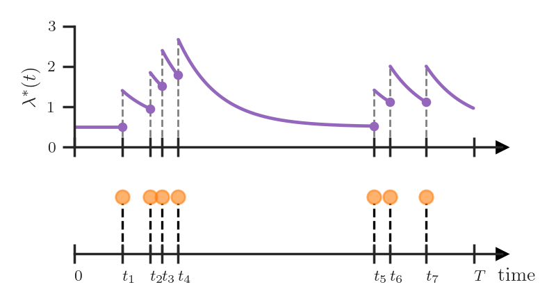
Another popular example is the self-exciting process (a.k.a. Hawkes process) with the conditional intensity function
\[\lambda^*(t) = \mu + \sum_{t_j \in \mathcal{H}_t} \alpha \exp(-(t - t_j))\]As we see above, the intensity increases by \(\alpha\) whenever an event occurs and then exponentially decays towards the baseline level \(\mu\). Such an intensity function allows us to capture “bursty” event occurrences — events often happen in quick succession. For example, if a neuron fires in the brain, it’s likely that this neuron will fire again in the near future.
Both of the above examples could equivalently be specified using the conditional PDFs \(f_i^*\) or the hazard functions \(h_i^*\). However, their description in terms of the conditional intensity \(\lambda^*(t)\) is more elegant and compact — we don’t have to worry about the indices \(i\), and we can understand the properties of respective TPPs (such as global trend or burstiness) by simply looking at the definition of \(\lambda^*(t)\).
TPP as a counting process
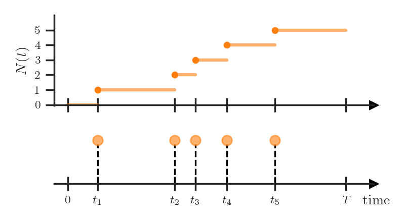
So far, we have represented TPP realizations as variable-length sequences, but this is not the only possible option. In many textbooks and (especially older) papers a TPP is defined as a counting process
It’s easy to see that this formulation is equivalent to the one we used before. We can represent an event sequence \(\boldsymbol{t} = (t_1, \dots, t_N)\) as a realization of a counting process by defining
\[N(t) = \sum_{i=1}^N \mathbb{I}(t_i \le t)\]where \(\mathbb{I}\) is the indicator function.
Last, we will consider is how to characterize the distribution of a counting process. Not surprisingly, the conditional intensity function \(\lambda^*(t)\) that we defined in the previous section will again come up here.
Like before, suppose that \(dt\) is an infinitesimal positive number. We will consider the expected change in \(N(t)\) during \(dt\) given the history of past events \(\mathcal{H}_t\), that is
By rearranging the above equation we could define the conditional intensity function as
\[\lambda^*(t) = \lim_{dt \to 0} \frac{\mathbb{E}[N(t + dt) - N(t) | \mathcal{H}_t]}{dt}\]which means, in simple words, that the conditional intensity is the expected number of events in a TPP per unit of time.
Summary
We have uncovered the mystery of the name “temporal point process”:
- Process — a TPP can be defined as a counting process
- Point — we can view each TPP realization $\boldsymbol{t} = (t_1, \dots, t_N)$ as a set of “points”
- Temporal — we can interpret the “points” $t_i$ as arrival times of events
We learned about different ways to specify a TPP, such as using the conditional intensity \(\lambda^*(t)\) or the conditional PDFs \(\{f_1^*, f_2^*, f_3^*, \dots\}\).
In the next post of this series, I will talk about how we can put this theory to practice and implement neural-network-based TPP models.
Acknowledgments
I would like to thank Johannes Klicpera for his feedback on this post.